Introduction to Fractal Geometry

At University, I did a full mathematics degree which covered around 36 modules – that’s quite a lot of maths! The weird thing about my degree (which is probably the case with most mathematics degrees?), is that most of the stuff we learnt was pretty darn old! To add some perspective, I think the most recent module was General Relativity which Einstein published in 1916. That’s strange! I know very little about maths which has been discovered/invented in the last 100 years!

With this in mind, I decided to look at some more recent stuff (1960’s/70’s) and bought a book on fractal geometry and chaos (James Gleick, Chaos: Making a New Science). It’s a popular Science book which is great as an introduction to the subject in terms of naming the key players and outlining the big ideas. As someone interested in mathematics (I never call myself a mathematician, as to me, this is someone who has or does contribute to the field), I needed to ‘branch out’ for a more in-depth understanding.

In this post, I’ll try to explain some of the basic mathematical principles behind Fractal Geometry from an IB/A-Level perspective. My knowledge only extends across two books, but hopefully this post will enable you to understand the most interesting and important stuff without spending weeks reading around the subject. I’ve enlisted the help of James Tanton and directed you to the Classic Iterated Functions Systems website to help with some of the explanations.

Introducing Fractal Geometry

Georg Cantor was one of the first mathematicians to study fractals in his quest to understand infinity (see my post on Infinite Set Theory and Cantor). The fractal he analysed was invented by Henry Smith in 1875 but it’s name is, unfortunately for Smith, attritibuted to Cantor. Below is an image of the Cantor set.

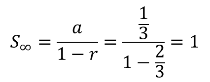
As you can see, Smith simply took a straight line and cut the middle third out of it. He then took the middle third out of the two lines remaining and so on ad infinitum (Latin phrase which means “to infinity). The act of repeating the same process over and over again is called iteration. If we think about all of the lengths taken away from each line then we end up with a simple geometric series.

1/3 + 2/9 + 4/27 + 8/81 + 16/243 + …

If you add up all of these lengths forever, you’ll never quite reach 1. Which makes sense because you can’t take away more length than you originally started with.

To show this, note that the common ratio is less than one (r = 2/3), so we can utilize the Infinite Sum formula for Geometric Series to add the terms. (First term, a = 1/3)

So why did Cantor analyse this set? In his time, little was known about fractals – both in a purely mathematical sense and in terms of how they connect to reality. Cantor simply used this fractal as an example of a particular type of set with special properties (a nowhere dense set) – nothing much to do with the “standard” mathematics of fractals today.

The Koch Snowflake is another example of a common fractal constructed by Helge von Koch in 1904.

If we just look at the top section of the snowflake. You can see that the iteration process requires taking the middle third section out of each line and replacing it with an equilateral triangle (bottom base excluded) with lengths that are equal to the length extracted.

It’s interesting to think about the perimeter and area of the Koch Snowflake.

Perimeter for the sections above:  Step 0 – 1, Step 1 (Generator Step) – 4/3 ≈ 1.333, Step 2 – 16/9 ≈ 1.777, Step 3 –  64/27 ≈ 2.370, Step 4 – 256/81 ≈ 3.160, Step 5 – 1024/243 ≈ 4.214 etc.

Since the Koch Snowflake is made up of 3 of these sections, just mutliply each of the numbers above by three. E.g. Perimeter of Snowflake at Step 4 ≈ 3 x 3.160 = 9.480.

After every iteration, the perimeter increases by a factor of 4/3  and will continue to increase in this way for an infinite number of iterations. i.e. it is not bounded by a certain value.

In contrast, the area of the snowflake is bounded i.e. no matter how many iterations you do, it will never surpass a certain point. Since it would take me quite a while to show this with diagrams and equations etc, let me point you to the site: Classic Iterated Function Systems which does it very clearly. Note in the second to last line on the page, the upper bound of the area is 8/5 of the original area.

Even without knowing much about fractals, at this point you’ve got to be intrigued by their beauty and complexity!

It gets better…

When you think about what the Koch snowflake actually is, how do you define something which is made up of an infinite number of line segments? Can we put in into the same class as 2-D shapes or would we classify it as a curve?

This is where the idea of a Fractal Dimension comes into play. So does the Koch Snowflake have a dimension of one or two or is it something else entirely? It turns out that you can compute the fractal dimension of a shape using a method which has been extremely well explained by Dr. James Tanton (see more brilliant videos made by Dr. Tanton at his website: Thinking Mathematics).

How awesome is that? We’re now considering shapes which have a dimension in between the “standard” dimensions. The fractal dimension of the Koch Curve for example is 1.2619! I have to admit, at first I was a bit wary about the term “size” in James’ video, after all, we have no formal definition of the word size. After a bit of thinking, I decided to accept this on the grounds that at least we know that we’re not looking at shapes with a size of zero and thus we can divide by the size in the equation.

Whilst I’m reluctant to write down a formula because I like the way James explains it, I’ve decided to do it anyway in the hope that people have a solid enough understanding of how to find the fractal dimension without the formula.

As a quick exercise, you may want to verify that the fractal dimension of the Cantor set is 0.6309.

Big Question 1: Why does this matter? What’s the point?

As Benoit Mandelbrot said,

Uniform objects like boxes and buildings do not appear in nature.

Nature contains shapes and surfaces which are complicated, rough and jagged, not smooth and simple like the shapes which occur in Euclidean geometry. We needed a new way of thinking about how to study the shape of a cloud, a lightning bolt or a coastline.

Big Question 2: How do we relate fractal shapes to natures shapes?

If you think about the coastline of Britain, it’s shape is complicated, rough and jagged. Furthermore, when you zoom in on it, it looks similar close up to how it does when you view it from space. Hence it is fractal-like. But how would we possibly start to analyse it using fractal mathematics if no exact copies of itself fit on it?

Benoit Mandelbrot (1924-2010) was concerned with this very question. He trailed through early Geographical papers trying to understand how to connect fractal shapes to those in nature and stumbled across a paper written by Lewis Richardson on, “How long is the coastline of Britain?” Mandelbrot determined a way of finding  the fractal dimension of a coastline using a box-counting technique given the data provided in Richardson’s paper.

Image produced by Alexis Monnerot-Dumaine: Prokofiev

You essentially cover the shape with a grid of squares and count how many squares the shape passes through and then do this again with a grid of smaller squares (the smaller the squares, the more accurate the calculation will be). Let’s say on the grid of larger squares, the shape passes through 40 squares and on the smaller grid, it passes through 218 squares. Dividing 218/40 gives you an approximate answer which is equivalent to the Number of Copies of itself which fit inside/on the shape in the numerator of the above formula. You can then easily calculate the length scale factor between the size of the smaller grid squares and the size of the larger grid squares (Note that the 218/40 is only approximate – as you decrease the size of the squares, you get a better approximation of the fractal dimension).

Apparently, if you do this for the coastline of Britain, you find that it has a fractal dimension which is similar to that of the Koch Curve! So Helge von Koch created a shape in 1904 which is essentially a model of the coastline of Britain – how cool is that!

We saw earlier that if you consider the actual Koch Curve (which has an infinite number of iterations – not just the 4th or 5th step), then the perimeter of it is infinite. So is the perimeter of the British Coastline infinite?

This is known as the coastline paradox. We can get an approximate value for the perimeter of the British Coastline (around 12,000 km) but this is based on how it was measured. If you went round the coastline with a 30 cm ruler, you’d find that you could’t meausure it accurately because it would be too “jagged.” Hence, you use a 15 cm ruler but it is still too jagged to measure accurately and you’d under measure it. In principle, you could keep on measuring it with a smaller and smaller measuring device and keep getting a larger and larger perimeter.

Having said this, I’m not sure if I agree on the infinite length of the coastline because I don’t think you could continue to zoom in on it forever like you could with the Koch Curve. I’m not sure on this but I believe that the most fundamental particles that we know of are quarks, neutrinos and electrons (I’m not sure if we know how small these actually are???). If we continued to zoom in on the coastline then at some point we’d get down to the fundamental particles and we wouldn’t be able to go any further. Thus if we had a device which could measure the number of quarks around the coastline, then we’d surely have a large, but finite answer. Of course, I’m assuming that there aren’t even smaller particles than quarks but I guess all that we can do is go with what we currently know.

Anyhow, that’s it for the first post on Fractal Geometry. Looking forward to writing some more on Fractal Geometry soon! I would love feedback on the last paragraph – do people agree or disagree?